View this notebook on GitHub or run it yourself on Binder!

---

Link Plots to Features

Rubicon_ml makes it easy to log plots with features and artifacts. In this example we’ll walk through creating a feature dependency plot using the shap package and saving it to an artifact.

Before getting started, we’ll have to install some dependencies for this example.

! pip install matplotlib kaleido Pillow shap "numba>=0.56.2"

Requirement already satisfied: matplotlib in /Users/nvd215/mambaforge/envs/rubicon-ml-dev/lib/python3.10/site-packages (3.6.1)
Requirement already satisfied: kaleido in /Users/nvd215/mambaforge/envs/rubicon-ml-dev/lib/python3.10/site-packages (0.2.1)
Requirement already satisfied: Pillow in /Users/nvd215/mambaforge/envs/rubicon-ml-dev/lib/python3.10/site-packages (9.2.0)
Requirement already satisfied: shap in /Users/nvd215/mambaforge/envs/rubicon-ml-dev/lib/python3.10/site-packages (0.41.0)
Requirement already satisfied: numba>=0.56.2 in /Users/nvd215/mambaforge/envs/rubicon-ml-dev/lib/python3.10/site-packages (0.56.2)

Set up

First lets create a Rubicon project and create a pipeline with rubicon_ml.sklearn.pipeline.

import shap
import sklearn
from sklearn.datasets import load_wine
from sklearn.ensemble import GradientBoostingRegressor
from sklearn.preprocessing import StandardScaler

from rubicon_ml import Rubicon
from rubicon_ml.sklearn import make_pipeline


rubicon = Rubicon(persistence="memory")
project = rubicon.get_or_create_project("Logging Feature Plots")

X, y = load_wine(return_X_y=True)

reg = GradientBoostingRegressor(random_state=1)
pipeline = make_pipeline(project, reg)

pipeline.fit(X, y)

RubiconPipeline(project=<rubicon_ml.client.project.Project object at 0x167a37c40>,
                steps=[('gradientboostingregressor',
                        GradientBoostingRegressor(random_state=1))])

In a Jupyter environment, please rerun this cell to show the HTML representation or trust the notebook.
On GitHub, the HTML representation is unable to render, please try loading this page with nbviewer.org.

Generating Data

After fitting the pipeline, using shap.Explainer we can generate shap values to later plot. For more information on generating shap values with shap.explainer, check the documentation here.

explainer = shap.Explainer(pipeline[0])
shap_values = explainer.shap_values(X)

Plotting

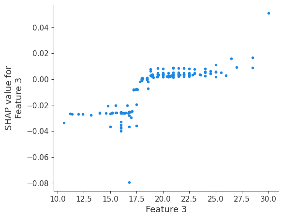
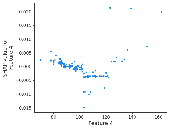
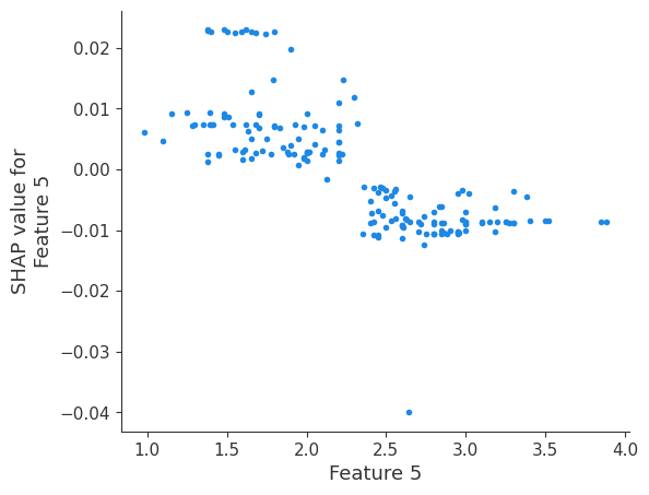
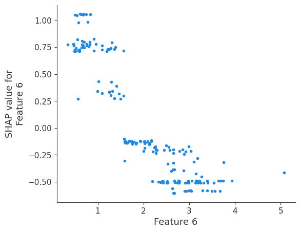
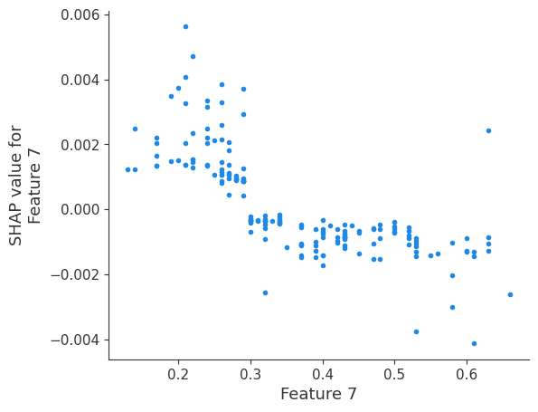
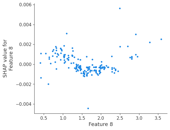
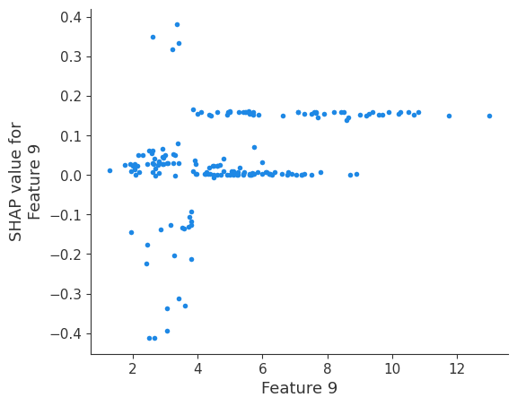
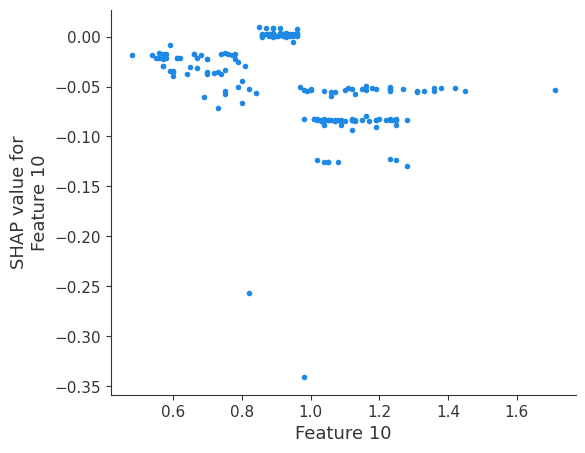
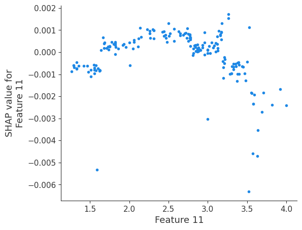
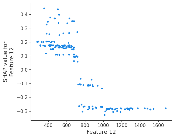
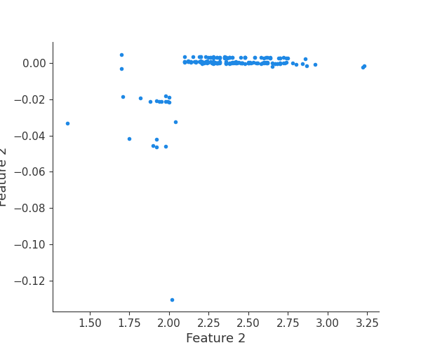
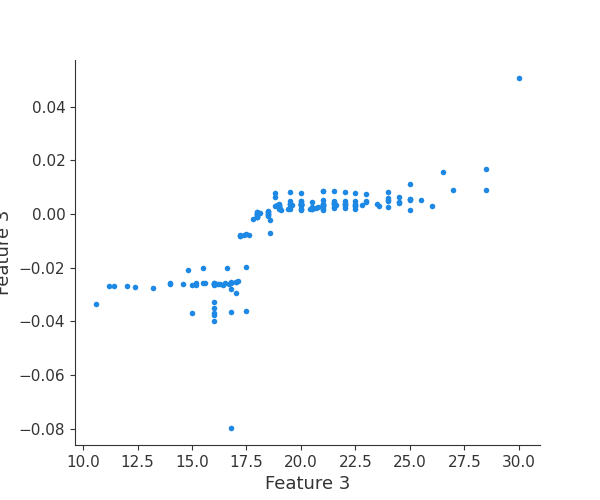
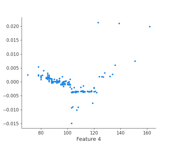
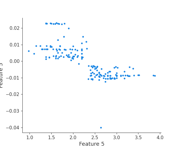
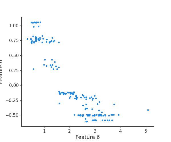
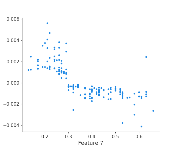
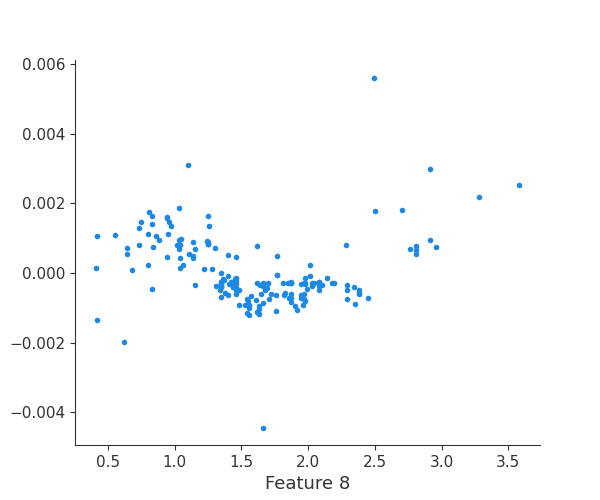
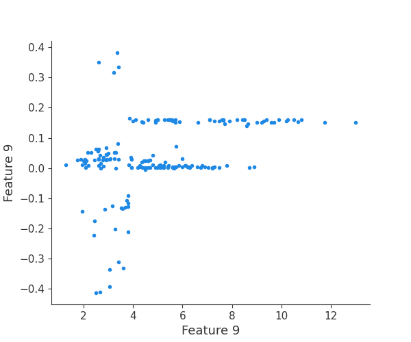
The generated shap_values from the above cell can be passed to a shap.depence_plot to generate a dependence plot. pl.gcf() allows the plot generated by shap to be saved to a variable. Using the matplotlib and io libraries, shap plots can be saved to a byte representation. Here, a feature and its plot are both logged withrubicon_ml.Features and rubuicon_ml.Artifact respectively. These features and artifacts are logged to the same rubicon_ml.Experiment that was created by calling pipeline.fit.

import io

import matplotlib.pyplot as pl


experiment = pipeline.experiment

for i in range(reg.n_features_in_):
    feature_name = f"feature {i}"
    experiment.log_feature(name=feature_name, tags=[feature_name])

    shap.dependence_plot(i, shap_values, X, interaction_index=None, show=False)

    fig = pl.gcf()
    buf = io.BytesIO()
    fig.savefig(buf, format="png")
    buf.seek(0)

    experiment.log_artifact(
        data_bytes=buf.read(), name=feature_name, tags=[feature_name],
    )

    buf.close()

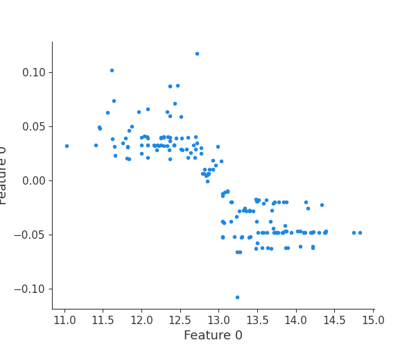
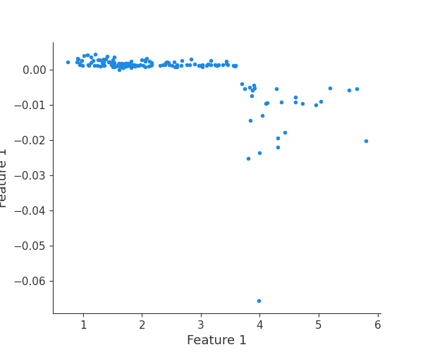
Retrieving your logged plot and features programmatically

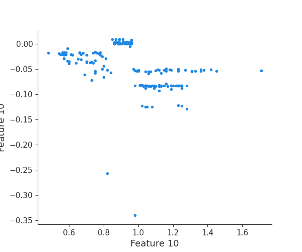
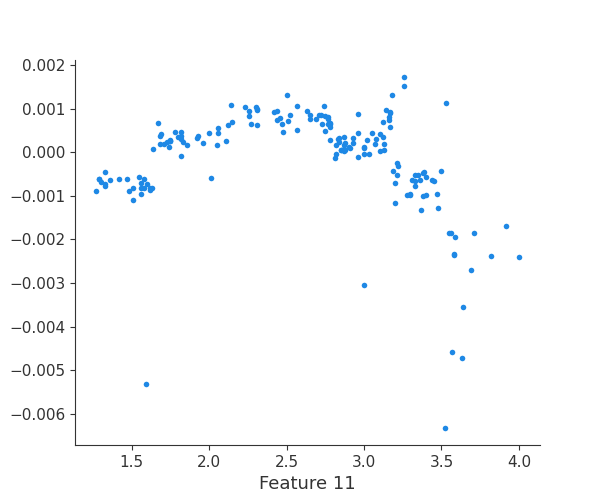
Finally, we can retrieve a feature and its associated artifact plot using the name argument. We’ll retrieve each artifact based on the names of the features logged. With IO and PIL, after retrieving the PNG byte representation of the plot, the plot can be rendered as a PNG image.

import io

from PIL import Image


experiment = pipeline.experiment

for feature in experiment.features():
    artifact = experiment.artifact(name=feature.name)

    buf = io.BytesIO(artifact.data)
    scatter_plot_image = Image.open(buf)

    print(feature.name)
    display(scatter_plot_image)

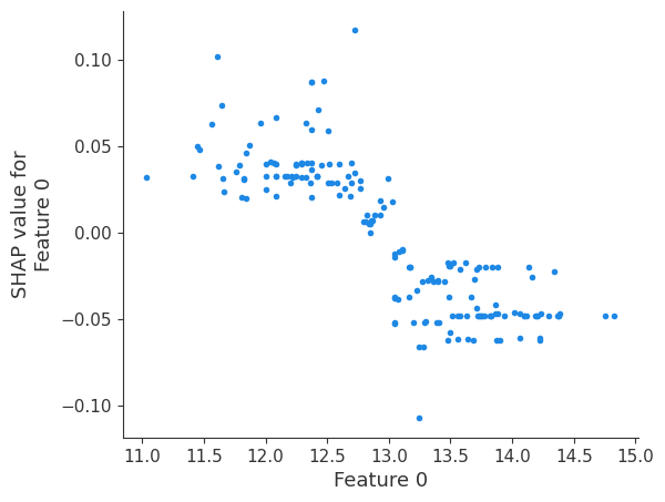
feature 0

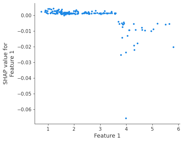
feature 1

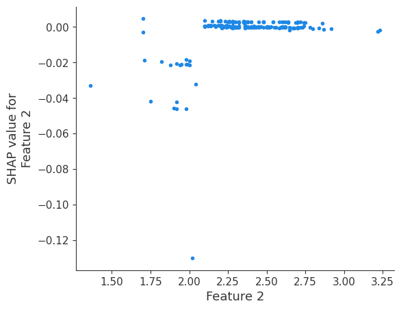
feature 2

feature 3

feature 4

feature 5

feature 6

feature 7

feature 8

feature 9

feature 10

feature 11

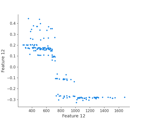
feature 12